Backprojection

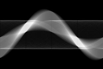
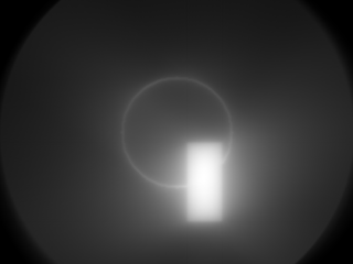
Fig. 1: Input image (left); sinogram (middle); backprojected image (right).

The goal of this exercise is to implement projection and backprojection algorithms and use them to reconstruct an image from a finite number of projections.

A well-known application of this principle is image reconstruction in computed tomography (CT).

Projection

Start by creating an input image similar to the one shown in Fig. 1 (left). You may also create a different test image if you prefer.

Next, compute projections of the input image for a set of angles in the interval $[0^{\circ },180^{\circ })$ using a step of $1^{\circ }$.

A projection is obtained by summing the pixel brightness values along parallel lines. Note that these sums can be greater than $255$, so choose an appropriate data type for the cv::Mat used to store the projection values.

A single projection forms a one-dimensional vector.

Computing projections directly for many different angles would be inconvenient. Instead, use a simple approach:

1. Rotate the input image by the required angle.
2. Compute the projection of the rotated image along the $x$-axis.
3. Store the resulting projection vector.

Repeating this procedure for all angles produces a set of projection vectors. These vectors can be arranged as rows or columns of a two-dimensional image called a sinogram (see Fig. 1, middle).

Backprojection

The original image can be approximately reconstructed from the set of projections using backprojection.

For each projection:

1. Take the one-dimensional projection vector.
2. Create an image in which this vector is copied repeatedly across the image.
3. Rotate the resulting image back by the angle at which the corresponding projection was acquired.
4. Add the rotated image to an accumulation image.

After processing all projections, the accumulated pixel values form the backprojected image.

The result is shown in Fig. 1 (right). Notice the clearly visible circular structure and the characteristic blurring caused by simple, unfiltered backprojection.