Introduction to OpenCV – Digital Image Processing Exercises
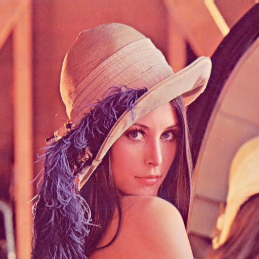
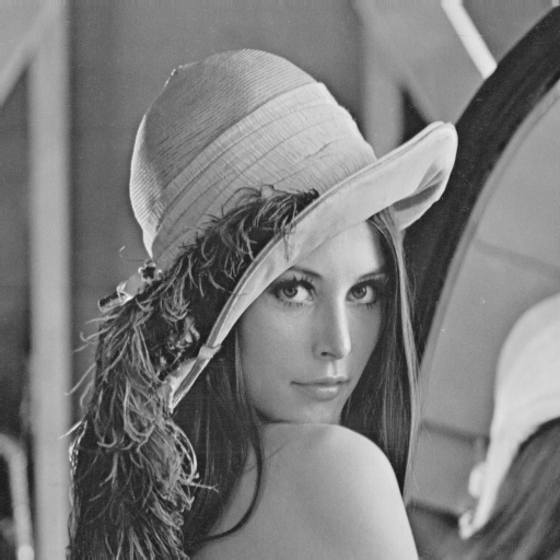
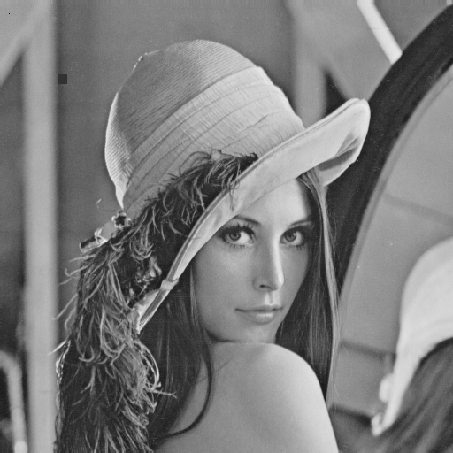
Figure: Color image of Lena (left); grayscale image of Lena (middle); grayscale image of Lena with modified pixel and drawn rectangle (right).
This repository contains introductory exercises for learning Digital Image Processing Course using C++ and OpenCV.
The goal of this exercise is to understand:
- How images are represented in memory
- How to load and convert images
- How to access and modify pixels
- How to create simple generated images
📚 Table of Contents
- Introduction to OpenCV – Digital Image Processing Exercises
- 📚 Table of Contents
- About OpenCV
- Project Overview
- How Images Are Stored in Memory
- Grayscale Memory Layout
- Color Image Memory Layout (BGR)
- Accessing Pixels Internally
- Loading Images
- Color Conversion
- Image Data Types
- Accessing Pixels
- Modifying Pixels
- Creating a Gradient Image
- Full Example Code
- How to Build and Run
- 🎓 Learning Outcomes
About OpenCV
We use the OpenCV library — an open-source C++ library containing many image processing and computer vision algorithms.
Key concepts:
- Most functionality lives inside the
cvnamespace - Images are stored using the
cv::Matdata type - Images are stored row by row in memory
- OpenCV uses
(not
)
Project Overview
This exercise demonstrates how to:
- Load a color image
- Convert it to grayscale
- Convert between data types
- Read and modify pixel values
- Draw a rectangle
- Generate a synthetic gradient image
How Images Are Stored in Memory
An image in OpenCV (cv::Mat) is essentially:
Pointer to data + width + height + type + step size
Images are stored row-major, meaning:
- The first row is stored first in memory
- Then the second row
- Then the third row
- And so on…
Memory layout:
Row 0:  p(0,0)  p(0,1)  p(0,2)  ...  p(0,width-1)
Row 1:  p(1,0)  p(1,1)  p(1,2)  ...  p(1,width-1)
Row 2:  p(2,0)  p(2,1)  p(2,2)  ...  p(2,width-1)
...
Grayscale Memory Layout
Grayscale image type: CV_8UC1
- 8 bits per pixel
- 1 channel
- Each pixel = 1 byte
Example (3×4 image):
Image:

[  10   20   30   40 ]
[  50   60   70   80 ]
[  90  100  110  120 ]
Memory layout (linear):
10 20 30 40 50 60 70 80 90 100 110 120
Access formula:
address = base + y * step + x
Where:
y= row indexx= column indexstep= number of bytes per row
Color Image Memory Layout (BGR)
Color image type: CV_8UC3
- 8 bits per channel
- 3 channels per pixel
- Each pixel = 3 bytes
- Order =
Example pixel:
Blue = 10
Green = 20
Red = 30
Memory storage:
[10][20][30]
Example (2×2 image):
Pixel(0,0)  Pixel(0,1)
Pixel(1,0)  Pixel(1,1)
Memory layout:
B00 G00 R00  B01 G01 R01
B10 G10 R10  B11 G11 R11
Linear memory:
p(0,0)B p(0,0)G p(0,0)R
p(0,1)B p(0,1)G p(0,1)R
p(1,0)B p(1,0)G p(1,0)R
p(1,1)B p(1,1)G p(1,1)R
Once again, OpenCV uses

Accessing Pixels Internally
When you write:
gray.at<uchar>(y, x);
OpenCV internally computes:
data + y * step + x * element_size
For:
- Grayscale → element_size = 1
- Color → element_size = 3
This is why using correct type (uchar, float, Vec3b) is critical.
Loading Images
To open an image, we use cv::imread function that returns an image that we can store in a variable. Images can be color or grayscale. Most of our algorithms will use grayscale images. The following code reads image in color and grayscale variant and stores them in two different variables.
cv::Mat src_8uc3_img = cv::imread("images/lena.png", cv::IMREAD_COLOR);
cv::Mat src_8uc1_img = cv::imread("images/lena.png", cv::IMREAD_GRAYSCALE);
Note: If you load image using
cv::IMREAD_GRAYSCALE, you don’t have to deal with color conversion described below.
Naming convention
| Variable | Meaning |
|---|---|
| 8U | 8-bit unsigned integer (uchar) |
| C3 | 3 channels (color image) |
| C1 | 1 channel (grayscale image) |
That means:
8UC3 → 8-bit, unsigned, 3-channel (color)
8UC1 → 8-bit, unsigned, 1-channel (grayscale)
Color Conversion
We can convert a color image to grayscale using:
cv::cvtColor(src_8uc3_img, gray_8uc1_img, cv::COLOR_BGR2GRAY);
And again, OpenCV uses
We just converted color image src_8uc3_img to empty image gray_8uc1_img (you can create an empty image by declaring a variable, for example, as: cv::Mat gray_8uc1_img).
Image Data Types
When we load an image from a file, each pixel is represented using 8 bits of information (unsigned char in C++ that we can refer as uchar). Pixel values are in range 0 - 255.
In grayscale image, we have one uchar per pixel.
In color image, we have three uchars per pixel forming traditional RGB pixels (as we’ve seen OpenCV uses BGR format).
However, for some image processing operations, it is better to represent image using values in range 0.0 - 1.0.
Such values have to stored in real value data type.
For our use, it’ll be completely sufficient to use float data type for such representation.
To convert a grayscale image from 8 bits (uchar)representation to 32 bits (float) representation we use convertTo method of cv::Mat variable.
The parameters of the method are:
- output image
- output data type
- conversion scale
By default:
- Pixel type:
uchar - Range: 0-255
For some algorithms, it is better to use floating point values:
float- Range: 0.0-1.0
The method may be used as follows
gray_8uc1_img.convertTo(gray_32fc1_img, CV_32FC1, 1.0 / 255.0);
Explanation:
| Parameter | Meaning |
|---|---|
gray_32fc1_img | Output image |
CV_32FC1 | 32-bit float, 1 channel |
1.0 / 255.0 | Scaling factor |
Accessing Pixels
Since the main aim of this course is to implement image processing algorithms, we’ll need to access pixels of an image. To do so, we’ll us at method of the cv::Mat data type. This method is templated (it needs a type specifier in angle brackets before arguments).
Use the templated at<> method:
at<Type>(int y, int x)
Example:
uchar p1 = gray_8uc1_img.at<uchar>(y, x);
float p2 = gray_32fc1_img.at<float>(y, x);
cv::Vec3b p3 = src_8uc3_img.at<cv::Vec3b>(y, x);
Accessing color channels in p3:
p3[0]  // Blue
p3[1]  // Green
p3[2]  // Red
Print values of pixels:
printf( "p1 = %d\n", p1 );
printf( "p2 = %f\n", p2 );
printf( "p3[ 0 ] = %d, p3[ 1 ] = %d, p3[ 2 ] = %d\n", p3[ 0 ], p3[ 1 ], p3[ 2 ] );
We’re assigning a grayscale value (brightness) to the uchar variable p1. gray_8uc1_img has brightness values represented using 8 bits. As you can see, type specifier of at method is set to uchar.
It’s followed by y, and x variables that specify, at which position to read pixel value.
The same procedure is done in the case of gray_32fc1_img image, which uses 32 bits representation of brightness values.
The only difference is that we use float instead of uchar
data type.
To access color pixels in src_8uc3_img, we need to use cv::Vec3b.
This type holds three values (BGR) at once.
To access each color value, we use [] operator as is used in the above example.
Modifying Pixels
Another important operation with image pixels is, of course, setting a new pixel brightness. This is done again using at method. The only difference from the read operation is that we assign a new value to the method.
To change a pixel value:
gray_8uc1_img.at<uchar>(y, x) = 0; // set to black
We’ll use this notation very often.
Creating a Gradient Image
When implementing image processing algorithms, you’ll quite often need to go through all image pixels and perform some operation with brightness values.
To access all pixels, we usually use two nested for loops to iterate over all rows and in each row to iterate over all columns.
As an example, we’ll create a gradient image.
First, we crate a new image named gradient_8uc1_img with 50 rows and 256 columns and with CV_8UC1 pixel data type.
This means that image will use 8 bits as data representation (uchar) and one channel, so it’s essentially a grayscale image.
Then we iterate over all pixels and assign brightness value according to the column number.
We generate a synthetic image:
- Width: 256 pixels
- Height: 50 pixels
- Type: CV_8UC1
cv::Mat gradient_8uc1_img(50, 256, CV_8UC1);

for (int y = 0; y < gradient_8uc1_img.rows; y++) {
    for (int x = 0; x < gradient_8uc1_img.cols; x++) {
        gradient_8uc1_img.at<uchar>(y, x) = x;
    }
}
Result image after calling cv::imshow( "Gradient 8uc1", gradient_8uc1_img );:

This creates a horizontal gradient from black (0) to white (255).
Full Example Code
#include <stdio.h>
#include <opencv2/opencv.hpp>

int main( int argc, char *argv[] )
{
    cv::Mat src_8uc3_img = cv::imread( "images/lena.png", cv::IMREAD_COLOR ); // load color image from file system into Mat variable, this will be loaded using 8 bits (uchar)

    // declare variable to hold grayscale version of img variable, gray levels wil be represented using 8 bits (uchar)
    cv::Mat gray_8uc1_img;
    // declare variable to hold grayscale version of img variable, gray levels wil be represented using 32 bits (float)
    cv::Mat gray_32fc1_img;

    cv::cvtColor( src_8uc3_img, gray_8uc1_img, cv::COLOR_BGR2GRAY ); // convert input color image to grayscale one, CV_BGR2GRAY specifies direction of conversion
    gray_8uc1_img.convertTo( gray_32fc1_img, CV_32FC1, 1.0 / 255.0 ); // convert grayscale image from 8 bits to 32 bits, resulting values will be in the interval 0.0 - 1.0

    int x = 10, y = 15; // pixel coordinates

    uchar p1 = gray_8uc1_img.at<uchar>( y, x ); // read grayscale value of a pixel, image represented using 8 bits
    float p2 = gray_32fc1_img.at<float>( y, x ); // read grayscale value of a pixel, image represented using 32 bits
    cv::Vec3b p3 = src_8uc3_img.at<cv::Vec3b>( y, x ); // read color value of a pixel, image represented using 8 bits per color channel

    // print values of pixels
    printf( "p1 = %d\n", p1 );
    printf( "p2 = %f\n", p2 );
    printf( "p3[ 0 ] = %d, p3[ 1 ] = %d, p3[ 2 ] = %d\n", p3[ 0 ], p3[ 1 ], p3[ 2 ] );

    gray_8uc1_img.at<uchar>( y, x ) = 0; // set pixel value to 0 (black)

    // draw a rectangle
    cv::rectangle( gray_8uc1_img, cv::Point( 65, 84 ), cv::Point( 75, 94 ),
                   cv::Scalar( 50 ), cv::FILLED );

    // declare variable to hold gradient image with dimensions: width= 256 pixels, height= 50 pixels.
    // Gray levels wil be represented using 8 bits (uchar)
    cv::Mat gradient_8uc1_img( 50, 256, CV_8UC1 );

    // For every pixel in image, assign a brightness value according to the x coordinate.
    // This wil create a horizontal gradient.
    for ( int y = 0; y < gradient_8uc1_img.rows; y++ ) {
        for ( int x = 0; x < gradient_8uc1_img.cols; x++ ) {
            gradient_8uc1_img.at<uchar>( y, x ) = x;
        }
    }

    // diplay images
    cv::imshow( "Gradient 8uc1", gradient_8uc1_img );
    cv::imshow( "Lena gray 8uc1", gray_8uc1_img );
    cv::imshow( "Lena gray 32fc1", gray_32fc1_img );

    cv::waitKey( 0 ); // wait until keypressed

    return 0;
}
How to Build and Run
Option 1 - Using g++ on command line
$ g++ main.cpp -o app `pkg-config --cflags --libs opencv4`
$ ./app
Option 2 - Using CMake (inluded in the template for Linux)
In Visual Studio Code, have installed CMake plugin:
$ code --install-extension ms-vscode.cpptools
$ code --install-extension ms-vscode.cmake-tools
Then run project by pressing: Shift + F5.
Or run using command line:
$ mkdir build
$ cd build
$ cmake ..
$ make
$ ./app
🎓 Learning Outcomes
After completing this exercise, you should understand:
- How images are stored in memory (row-major order)
- Difference between 1-channel and 3-channel images
- Why OpenCV uses BGR
- How
cv::Matmanages memory - How pixel access translates to pointer arithmetic
- The foundation of implementing custom image processing algorithms
Convolution
In this exercise, we will implement a convolution algorithm. Convolution is a mathematical operation that combines two functions to produce a third function. In digital image processing, it is commonly used to implement various image filters.
In digital image processing, convolution usually takes the following form:
\[ (f * h)(x, y) = \sum\limits_{i=-k}^{k} \sum\limits_{j=-k}^{k} f(x - i, y - j) \cdot h(i, j) \, , \tag{1} \]
where \(f\) is and input image, \(h\) is a convolution matrix (mask), and \(k\) is the width of the convolution mask.
Convolution mask is a matrix usually of size \(3 \times 3\) or \(5 \times 5\). Some examples of convolution masks follow:
\[ \text{Box blur:} \quad\quad \frac{1}{9} \begin{bmatrix} 1 & 1 & 1 \\ 1 & 1 & 1 \\ 1 & 1 & 1 \end{bmatrix} \, , \tag{2} \]
\[ \text{Gaussian blur } 3 \times 3\text{:} \quad\quad \frac{1}{16} \begin{bmatrix} 1 & 2 & 1 \\ 2 & 4 & 2 \\ 1 & 2 & 1 \end{bmatrix} \, , \tag{3} \]
\[ \text{Gaussian blur } 5 \times 5\text{:} \quad\quad \frac{1}{256} \begin{bmatrix} 1 & 4 & 6 & 4 & 1 \\ 4 & 16 & 24 & 16 & 4 \\ 6 & 24 & 36 & 24 & 6 \\ 4 & 16 & 24 & 16 & 4 \\ 1 & 4 & 6 & 4 & 1 \end{bmatrix} \, . \tag{4} \]
Informally, convolution computes each output pixel as a weighted sum of the neighbouring pixels in the input image. The weights are given by the corresponding values of the convolution kernel.
When the kernel is centred close to the image boundary, some of its elements extend beyond the image. Without introducing an additional boundary-handling strategy, convolution therefore cannot be computed for these pixels. The width of this border depends on the kernel size. For a \(3 \times 3\) kernel, the border is \(1\) pixel wide, while for a \(5 \times 5\) kernel, it is \(2\) pixels wide.
Fig. 1 illustrates the convolution operation at a particular pixel location.
Fig. 1: An example of convolution operation at a pixel location.
Anisotropic Filtration
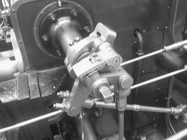
Fig. 1: Input image (left); filtered image after 1000 iterations (right).
In this exercise, we will implement anisotropic filtering of images.
Unlike Gaussian blur, anisotropic filtering smooths an image while preserving sharp edges. The method is based on the physical phenomenon of energy diffusion from regions of higher concentration to regions of lower concentration. In an image, the energy concentration can be represented, for example, by the brightness value of each pixel.
The pixels are arranged on a grid that forms a mesh network. Neighbouring pixels are connected by resistors, and their resistance, or equivalently their conductance, depends on the similarity of the connected pixels. The filtering process evolves over time. In each time step, a small amount of energy flows between neighbouring pixels. The process stops after a predefined number of iterations.
A model of a pixel neighbourhood is shown in Fig. 2. The conductances between neighbouring pixels can be computed as follows:
\[ \begin{aligned} c_{N_{i,j}}^{t} &= g \left(\left|\nabla_N I_{i,j}^{t}\right|\right) \\ c_{S_{i,j}}^{t} &= g \left(\left|\nabla_S I_{i,j}^{t}\right|\right) \\ c_{E_{i,j}}^{t} &= g \left(\left|\nabla_E I_{i,j}^{t}\right|\right) \\ c_{W_{i,j}}^{t} &= g \left(\left|\nabla_W I_{i,j}^{t}\right|\right) \, , \end{aligned} \tag{1} \]
where \(g\) is defined as
\[ g(\nabla I) = e^{\left(-\frac{\left| \nabla I\right|^2}{\sigma^2}\right)} \tag{2} \]
and \(\nabla_N I_{i,j} = I_{i,j-1} - I_{i,j}\). The gradients in the other directions are computed analogously (see Fig. 2).
In each iteration, the new value of a pixel is computed using the following formula:
where \(I_{i,j}^{t+1}\) is the new brightness value at coordinates \((i,j)\) at time \(t+1\), and \(I_{i,j}^{t}\) is the brightness value at the same coordinates at time \(t\).
Using Eq. (3), compute the new value of every pixel at time \(t+1\) from the image values at time \(t\). Note that this is not an in-place operation: the new values must be written to a separate output image.
For your experiments, use \(\sigma = 0.015\) and \(\lambda = 0.1\).
Fig. 2: A model of a pixel at coordinates \((i,j)\) with north (\(N\)), south (\(S\)), west (\(W\)), and east (\(E\)) neighbours.
Hint: Use the double data type to represent the input and output images.
Discrete Fourier Transform
Today’s exercise focuses on the implementation of the Discrete Fourier Transform (DFT). In the next lecture, we will implement the inverse transform.
The Fourier Transform computes the frequency spectrum of a given input image . This spectrum is denoted by ; it is a complex matrix with the same dimensions as the input image.
The basis function is defined as
To compute the basis function, it is useful to use Euler’s formula
Using this relation, the result can be split into real and imaginary parts:
The spectrum amplitude is computed as follows:
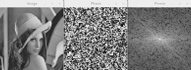
The phase is defined as
The power spectrum can be computed as
To display the power spectrum, first apply a logarithm to its values and then normalize them to the interval .
For a conventional visualization of the spectrum, swap the first and third quadrants, and also the second and fourth quadrants. This swap should be performed on both the real and imaginary parts of the computed spectrum. This will also be useful later when applying filters.
Hint: Use the double data type to represent the input image, the frequency spectrum values, and the phase.
Expected Output
Inverse Discrete Fourier Transform
In the previous lesson, we’ve implemented the Discrete Fourier Transform. Today, we’ll implement its inverse called the Inverse Discrete Fourier Transform (IDFT).
We want to transform the frequency spectrum back to its spatial domain , which is an image. The computation of the IDFT can be easily implemented using following formula
The basis is defined as
Notice that argument of is positive, so it’s different from the basis used in DFT.
To compute the basis, it’s advantageous to use Eulers formula .
Don’t forget that elements in the matrix are complex, so is the basis. Think for a while, what will be the result.
Hint: Use double data type as last time.
Filtering Using the Discrete Fourier Transform
In this exercise, we will implement simple filters using the results of the Discrete Fourier Transform (DFT).
An input image is often corrupted by noise, which is typically represented by high-frequency components in the frequency domain. One of the goals of this exercise is to create a filter that removes noise from the input image. Another task is to remove regular vertical bars from an image.
Noise Removal
As mentioned above, noise is typically represented by high frequencies in the frequency domain. In the previous exercises, we implemented both the transformation of an image into the frequency domain using the DFT and the inverse transformation back into the spatial domain using the IDFT. We will now introduce filtering into this processing pipeline.
In the frequency domain, we can apply several types of filters, including low-pass, high-pass, and band-pass filters. To remove noise, use a low-pass filter.
Recall that after the DFT, the low frequencies are located in the corners of the complex matrix, while the high frequencies are located near the centre. To make the filter easier to construct and apply, swap the first quadrant with the third and the second quadrant with the fourth, as shown schematically in Fig. 1.
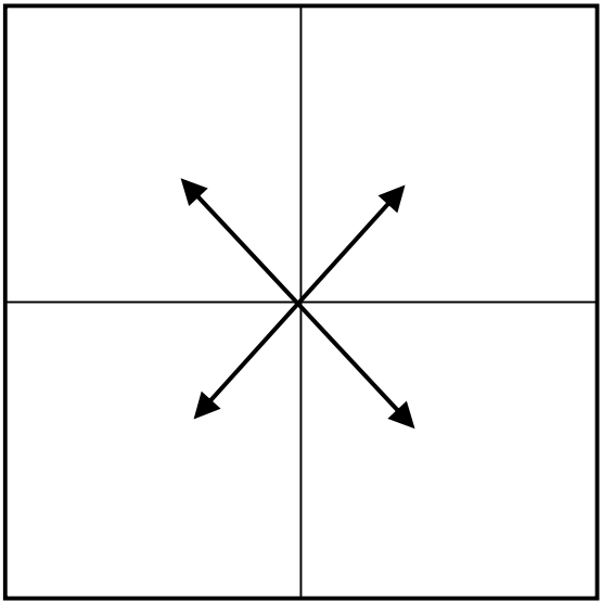
Fig. 1: Quadrant swap.
Next, create a circular mask that is white inside the circle and black outside it, as shown in Fig. 2.
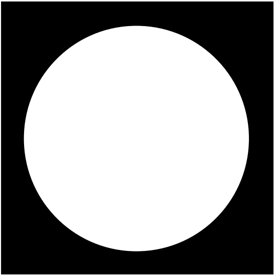
Fig. 2: Circular frequency-domain mask.
The diameter of the circle determines the strength of the filtering. Experiment with different diameters and observe how they affect the result.
To remove high frequencies using a low-pass filter, iterate over the pixels of the mask and set the corresponding values of the complex frequency-domain matrix to wherever the mask is black. For a high-pass filter, do the opposite and remove the frequencies inside the white circle.
After modifying the frequency-domain values, swap the quadrants back to their original positions and use the IDFT to transform the result back into the spatial domain.
An example of low-pass and high-pass filtering is shown in Fig. 3.
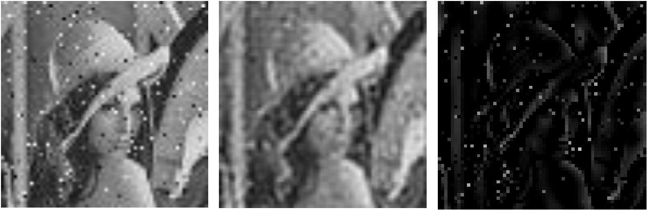
Fig. 3: Input image (left); low-pass filtered image (middle); high-pass filtered image (right).
Removing Regular Vertical Lines
The second task is slightly more complex. Your goal is to determine which frequencies correspond to the regular vertical lines in the input image.
The frequency-spectrum images provided on the exercise website can help you identify the relevant frequency components. By setting the appropriate parts of the complex frequency-domain matrix to , you can suppress the periodic pattern and obtain a result similar to the one shown in Fig. 4.
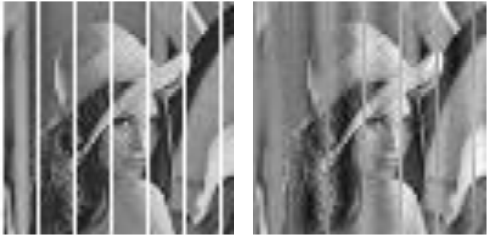
Fig. 4: Input image (left); image after removal of the vertical bars (right).
Removal of Geometric Distortion
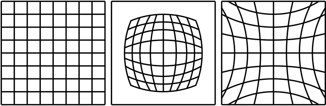
Fig. 1: Undistorted image, barrel distortion, and pincushion distortion.
Barrel and pincushion distortions are examples of radial distortion. One of the simplest ways to model these distortions is by transforming image coordinates.
Let represent the undistorted coordinates and the observed coordinates, i.e. the coordinates in the distorted image. Any radially symmetric distortion can be approximated using a Taylor series of the following form:
where , and , , are the radial distortion coefficients.
To make the coordinates independent of the image dimensions, and are dimensionless. In addition, to preserve radial symmetry, the origin of the coordinate system must be moved to the centre of the image. Coordinates with the required properties can be obtained as follows:
where
and the coordinates of the image centre are
where is the image width and is the image height.
The transformation from the coordinates in the reconstructed image to the corresponding coordinates in the original distorted image can then be written as
Process the output image pixel by pixel. For each output pixel , compute the corresponding coordinates in the input image.
In general, the resulting coordinates are real-valued, so an interpolation method must be used to obtain the pixel value. The simplest option is nearest-neighbour interpolation. For better results, use bilinear interpolation.
An example of the result obtained using this method is shown in Fig. 2.
Fig. 2: Original distorted image (left); image after removal of radial distortion (right).
Histogram Equalization
In this exercise, we will implement histogram equalization.
Sometimes, an image has a relatively narrow distribution of brightness values (see Fig. 1). Such an image has low contrast, which makes details difficult to distinguish. There are many techniques for improving image contrast; in this exercise, we will implement a simple one.
First, compute the histogram of the image. The histogram indicates how many pixels in the image have a particular brightness value . In our case, , where is the number of brightness levels in the image. For an 8-bit grayscale image, .
The histogram value for brightness level is defined as
where is the number of pixels with brightness value .
Next, compute the cumulative distribution function corresponding to the histogram:
Finally, compute the new brightness value using
where is the original brightness value, is the smallest non-zero value of the cumulative distribution function, and is the new brightness value.
To speed up the process, construct a simple look-up table (LUT) with entries. First, compute the transformed brightness value for every possible input value and store the results in the LUT. Then, iterate over the image and replace each brightness value with the corresponding value from the LUT.
Expected Output
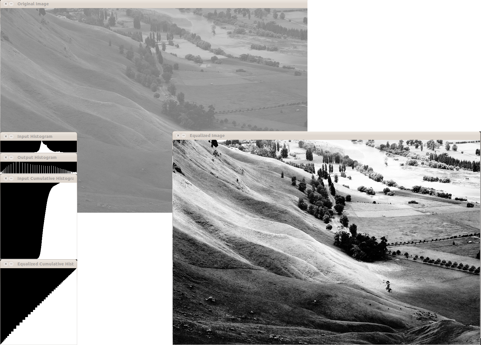
Fig. 1: An example of histogram equalization. Notice the input and output histograms and cumulative distribution functions.
Edge Detection
Image segmentation is an important task in image analysis. Its goal is to separate objects of interest from the image background. Since objects often differ from the background in color or brightness, segmentation can frequently be based on detecting object boundaries.
These boundaries correspond to edges—locations in the image where the color or brightness function changes significantly. Therefore, edges can be detected by analyzing derivatives of the image intensity function (see Fig. 1).
In this exercise, you will implement three basic edge-detection methods.
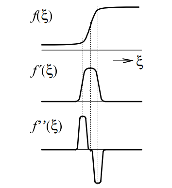
Fig. 1: The brightness function and its first and second derivatives.
First Derivative
As shown in Fig. 1, the absolute value of the first derivative is high at locations where an edge occurs.
The edge response can therefore be estimated using the derivatives
which describe changes in the brightness function in the and directions.
Since digital images are discrete, the derivatives are approximated by finite differences:
The edge magnitude is then computed as
Compute this value for every image pixel. If is greater than a chosen threshold, the pixel is considered to belong to an edge.
The result of this method, normalized for visualization, is shown in Fig. 4 (top right).
Second Derivative
Figure 1 also illustrates how an edge can be detected using the second derivative. Around an edge, the second derivative typically reaches a positive and a negative extremum, and the zero crossing between them indicates the edge location.
For this purpose, the Laplacian operator can be used.
As before, the brightness function is analyzed in the and directions:
The Laplacian is defined as
Because the image domain is discrete, the second derivatives are approximated using finite differences:
Substituting these expressions into the Laplacian gives
The result of this method, normalized for visualization, is shown in Fig. 4 (bottom left).
Sobel Operator
The Sobel operator is also based on differences between pixel values in the and directions. However, instead of using only two neighboring pixels, it estimates the edge response from a neighborhood.
The labeling of neighboring pixels is shown in Fig. 2.
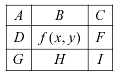
Fig. 2: Labeling of neighboring image pixels.
The Sobel kernels for the and directions are shown in Fig. 3.
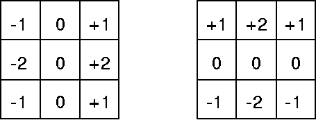
Fig. 3: Sobel kernels for the and directions.
Using the labels from Fig. 2, the horizontal and vertical responses are computed as
These formulas can be represented by convolution kernels, as shown in Fig. 3. Therefore, the Sobel response can be computed using image convolution.
The edge magnitude can then be obtained in the same way as for the first-derivative method:
The result of the Sobel operator is shown in Fig. 4 (bottom right).
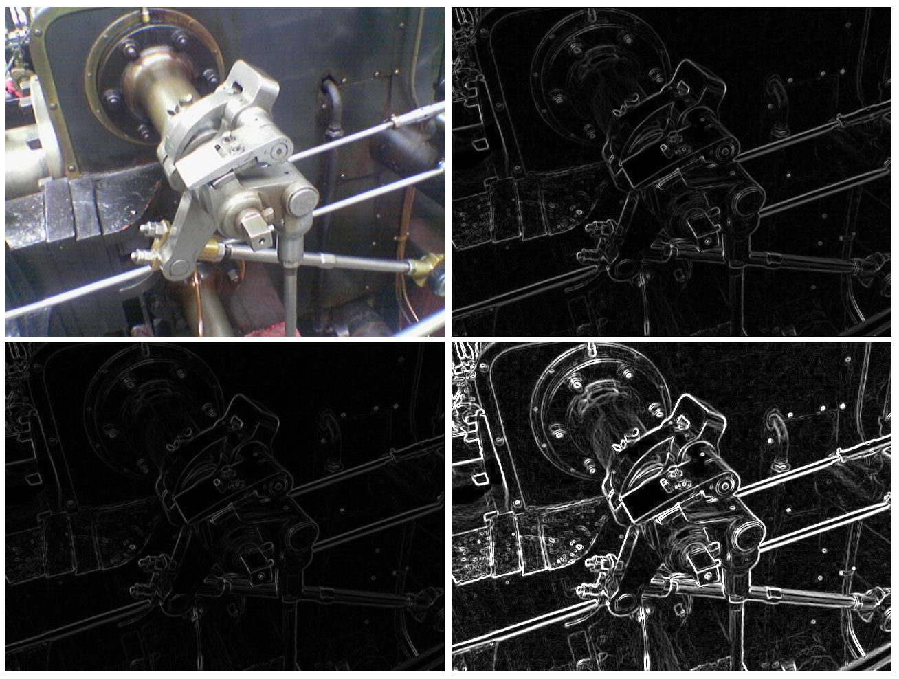
Fig. 4: Input image (top left); edges detected using the first derivative (top right), the second derivative (bottom left), and the Sobel operator (bottom right).
Edge Thinning and Double Thresholding
In this exercise, we will implement edge thinning followed by double thresholding to obtain clean, one-pixel-wide edges.
Non-Maximum Suppression
So far, we have used the Sobel operator and other convolution-based operators to detect edges in images. In this exercise, we will instead compute the image derivatives using central differences:
and
The resulting edges are typically several pixels wide. Our goal is to reduce them to one-pixel-wide contours. This process is called edge thinning, and we will achieve it using non-maximum suppression.
Non-maximum suppression removes values that are not local maxima. In other words, a pixel is preserved only if its edge magnitude is greater than the magnitudes of its relevant neighboring pixels.
In a one-dimensional case, a value is retained only if it satisfies
Thus, the value at position must be greater than both its left and right neighbors.
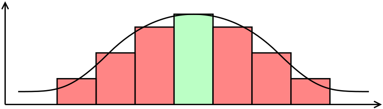
Fig. 1: Example of one-dimensional non-maximum suppression. The green bar represents a local maximum and is preserved. The red bars are not local maxima and are therefore set to zero.
The two-dimensional case is more complex because the neighboring values must be compared in the direction of the edge gradient.
The values and are therefore computed by linear interpolation of nearby pixel values, as illustrated in Fig. 2.
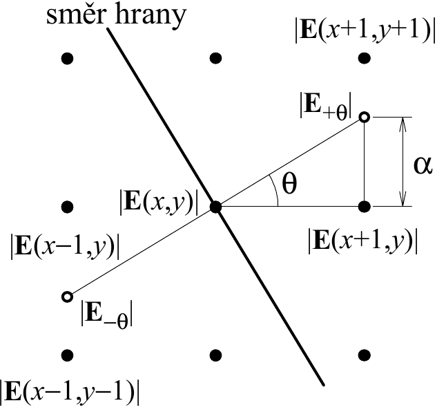
Fig. 2: An edge and the corresponding gradient values. The diagram uses a Cartesian coordinate system with the origin in the bottom-left corner. OpenCV images use the origin in the top-left corner, so adapt the coordinate handling accordingly.
The interpolated values are computed as
and
The current pixel is preserved only if its edge magnitude is greater than the interpolated edge magnitudes on both sides of the edge direction.
Double Thresholding
After non-maximum suppression, the image contains edge magnitudes only near the centers of detected edges. The next step is to distinguish meaningful edges from small responses caused by noise or minor image variations.
For this purpose, use two experimentally chosen thresholds, and , such that
For each edge magnitude :
- if , mark the pixel at as a strong edge pixel and set the corresponding output value to ;
- if , treat the pixel as a weak edge pixel;
- preserve a weak edge pixel only if it is connected to a pixel that has already been classified as an edge.
This procedure can be implemented conveniently using a recursive function. Whenever a pixel is classified as an edge, recursively examine its top, bottom, left, and right neighbors and include weak edge pixels that are connected to it.
Backprojection
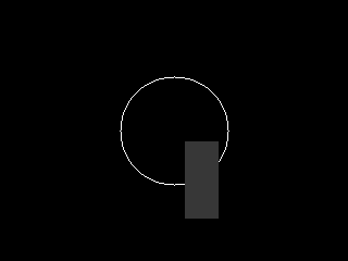
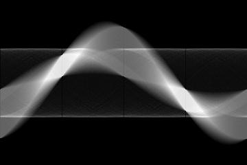
Fig. 1: Input image (left); sinogram (middle); backprojected image (right).
The goal of this exercise is to implement projection and backprojection algorithms and use them to reconstruct an image from a finite number of projections.
A well-known application of this principle is image reconstruction in computed tomography (CT).
Projection
Start by creating an input image similar to the one shown in Fig. 1 (left). You may also create a different test image if you prefer.
Next, compute projections of the input image for a set of angles in the interval using a step of .
A projection is obtained by summing the pixel brightness values along parallel lines. Note that these sums can be greater than , so choose an appropriate data type for the cv::Mat used to store the projection values.
A single projection forms a one-dimensional vector.
Computing projections directly for many different angles would be inconvenient. Instead, use a simple approach:
- Rotate the input image by the required angle.
- Compute the projection of the rotated image along the -axis.
- Store the resulting projection vector.
Repeating this procedure for all angles produces a set of projection vectors. These vectors can be arranged as rows or columns of a two-dimensional image called a sinogram (see Fig. 1, middle).
Backprojection
The original image can be approximately reconstructed from the set of projections using backprojection.
For each projection:
- Take the one-dimensional projection vector.
- Create an image in which this vector is copied repeatedly across the image.
- Rotate the resulting image back by the angle at which the corresponding projection was acquired.
- Add the rotated image to an accumulation image.
After processing all projections, the accumulated pixel values form the backprojected image.
The result is shown in Fig. 1 (right). Notice the clearly visible circular structure and the characteristic blurring caused by simple, unfiltered backprojection.