Discrete Fourier Transform

Today’s exercise focuses on the implementation of the Discrete Fourier Transform (DFT). In the next lecture, we will implement the inverse transform.

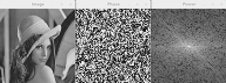
The Fourier Transform computes the frequency spectrum of a given input image $f$. This spectrum is denoted by $F$; it is a complex matrix with the same dimensions as the input image.

$$F(k,l)=\sum _{m=0}^{M-1}\sum _{n=0}^{N-1}f(m,n){\phi }_{k,l}(m,n).\text{\hspace{1em}(1)}$$

The basis function ${\phi }_{k,l}$ is defined as

$${\phi }_{k,l}(m,n)=\frac{1}{\sqrt{MN}}{e}^{-i2\pi \left(\frac{mk}{M}+\frac{nl}{N}\right)},k=0,1,\dots ,M-1,l=0,1,\dots ,N-1.\text{\hspace{1em}(2)}$$

To compute the basis function, it is useful to use Euler’s formula

$$e^{ix}=\cos (x)+i\sin (x).$$

Using this relation, the result can be split into real and imaginary parts:

$$F(k,l)=R(k,l)+I(k,l).\text{\hspace{1em}(3)}$$

The spectrum amplitude $|F(k,l)|$ is computed as follows:

$$|F(k,l)|=\sqrt{R^2(k,l)+I^2(k,l)}.\text{\hspace{1em}(4)}$$

The phase $\Phi (k,l)$ is defined as

$$\Phi (k,l)=\arctan \left(\frac{I(k,l)}{R(k,l)}\right).\text{\hspace{1em}(5)}$$

The power spectrum $P(k,l)$ can be computed as

$$P(k,l)=|F(k,l){|}^2.$$

To display the power spectrum, first apply a logarithm to its values and then normalize them to the interval $⟨0,1⟩$.

For a conventional visualization of the spectrum, swap the first and third quadrants, and also the second and fourth quadrants. This swap should be performed on both the real and imaginary parts of the computed spectrum. This will also be useful later when applying filters.

Hint: Use the double data type to represent the input image, the frequency spectrum values, and the phase.

Expected Output