Edge Detection

Image segmentation is an important task in image analysis. Its goal is to separate objects of interest from the image background. Since objects often differ from the background in color or brightness, segmentation can frequently be based on detecting object boundaries.

These boundaries correspond to edges—locations in the image where the color or brightness function changes significantly. Therefore, edges can be detected by analyzing derivatives of the image intensity function (see Fig. 1).

In this exercise, you will implement three basic edge-detection methods.

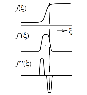
Fig. 1: The brightness function and its first and second derivatives.

First Derivative

As shown in Fig. 1, the absolute value of the first derivative is high at locations where an edge occurs.

The edge response can therefore be estimated using the derivatives

$$\frac{\partial f}{\partial x}\text{and}\frac{\partial f}{\partial y},$$

which describe changes in the brightness function in the $x$ and $y$ directions.

Since digital images are discrete, the derivatives are approximated by finite differences:

$$\begin{array}{rl}{f}_x(x,y)& =f(x+1,y)-f(x,y),\\ f_y(x,y)& =f(x,y+1)-f(x,y).\end{array}\text{\hspace{1em}(1)}$$

The edge magnitude is then computed as

$$e(x,y)=\sqrt{f_x^2(x,y)+f_y^2(x,y)}.\text{\hspace{1em}(2)}$$

Compute this value for every image pixel. If $e(x,y)$ is greater than a chosen threshold, the pixel is considered to belong to an edge.

The result of this method, normalized for visualization, is shown in Fig. 4 (top right).

Second Derivative

Figure 1 also illustrates how an edge can be detected using the second derivative. Around an edge, the second derivative typically reaches a positive and a negative extremum, and the zero crossing between them indicates the edge location.

For this purpose, the Laplacian operator can be used.

As before, the brightness function is analyzed in the $x$ and $y$ directions:

$$f_{xx}=\frac{{\partial }^{2}f(x,y)}{\partial x^2},f_{yy}=\frac{{\partial }^{2}f(x,y)}{\partial y^2}.$$

The Laplacian is defined as

$${\nabla }^{2}f(x,y)=f_{xx}(x,y)+f_{yy}(x,y).\text{\hspace{1em}(3)}$$

Because the image domain is discrete, the second derivatives are approximated using finite differences:

$$\begin{array}{rl}{f}_{xx}(x,y)& =f(x-1,y)-2f(x,y)+f(x+1,y),\\ f_{yy}(x,y)& =f(x,y-1)-2f(x,y)+f(x,y+1).\end{array}\text{\hspace{1em}(4)}$$

Substituting these expressions into the Laplacian gives

$${\nabla }^{2}f(x,y)=f(x-1,y)+f(x+1,y)+f(x,y-1)+f(x,y+1)-4f(x,y).\text{\hspace{1em}(5)}$$

The result of this method, normalized for visualization, is shown in Fig. 4 (bottom left).

Sobel Operator

The Sobel operator is also based on differences between pixel values in the $x$ and $y$ directions. However, instead of using only two neighboring pixels, it estimates the edge response from a $3\times 3$ neighborhood.

The labeling of neighboring pixels is shown in Fig. 2.

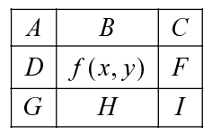
Fig. 2: Labeling of neighboring image pixels.

The Sobel kernels for the $x$ and $y$ directions are shown in Fig. 3.

Fig. 3: Sobel kernels for the $x$ and $y$ directions.

Using the labels from Fig. 2, the horizontal and vertical responses are computed as

$$\begin{array}{rl}{f}_x(x,y)& =(C-A)+2(F-D)+(I-G),\\ f_y(x,y)& =(A-G)+2(B-H)+(C-I).\end{array}\text{\hspace{1em}(6)}$$

These formulas can be represented by $3\times 3$ convolution kernels, as shown in Fig. 3. Therefore, the Sobel response can be computed using image convolution.

The edge magnitude can then be obtained in the same way as for the first-derivative method:

$$e(x,y)=\sqrt{f_x^2(x,y)+f_y^2(x,y)}.\text{\hspace{1em}(7)}$$

The result of the Sobel operator is shown in Fig. 4 (bottom right).

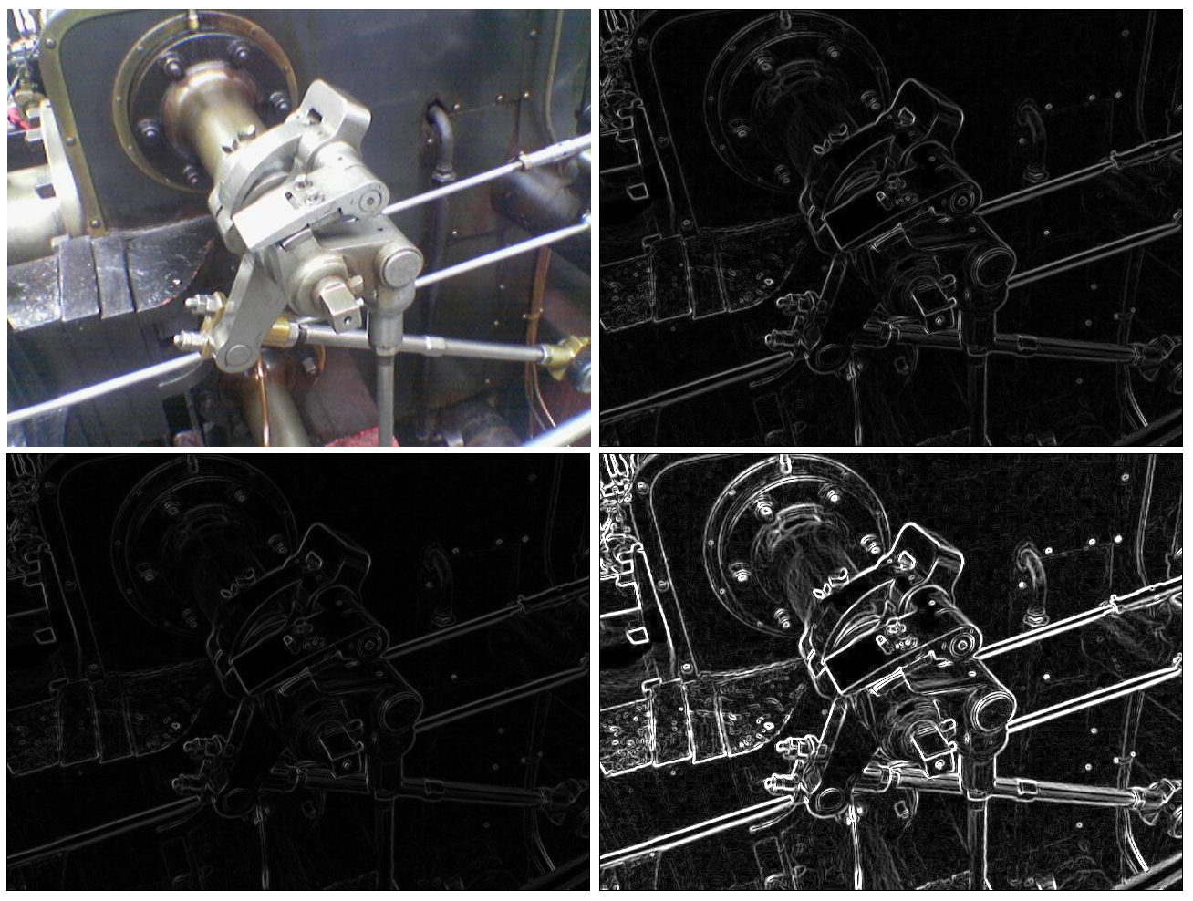
Fig. 4: Input image (top left); edges detected using the first derivative (top right), the second derivative (bottom left), and the Sobel operator (bottom right).