Histogram Equalization

In this exercise, we will implement histogram equalization.

Sometimes, an image has a relatively narrow distribution of brightness values (see Fig. 1). Such an image has low contrast, which makes details difficult to distinguish. There are many techniques for improving image contrast; in this exercise, we will implement a simple one.

First, compute the histogram of the image. The histogram indicates how many pixels in the image have a particular brightness value $i$. In our case, $i\in [0,L-1]$, where $L$ is the number of brightness levels in the image. For an 8-bit grayscale image, $L=256$.

The histogram value for brightness level $i$ is defined as

$$p(i)=n_i,\text{\hspace{1em}(1)}$$

where $n_i$ is the number of pixels with brightness value $i$.

Next, compute the cumulative distribution function corresponding to the histogram:

$$cdf(i)=\sum _{j=0}^i{n}_j.\text{\hspace{1em}(2)}$$

Finally, compute the new brightness value using

$$h(v)=\mathrm{round}\left(\frac{cdf(v)-cd{f}_{\min }}{\left(\text{width}\times \text{height}\right)-cd{f}_{\min }}\left(L-1\right)\right),\text{\hspace{1em}(3)}$$

where $v$ is the original brightness value, $cd{f}_{\min }$ is the smallest non-zero value of the cumulative distribution function, and $h(v)$ is the new brightness value.

To speed up the process, construct a simple look-up table (LUT) with $L$ entries. First, compute the transformed brightness value for every possible input value and store the results in the LUT. Then, iterate over the image and replace each brightness value with the corresponding value from the LUT.

Expected Output

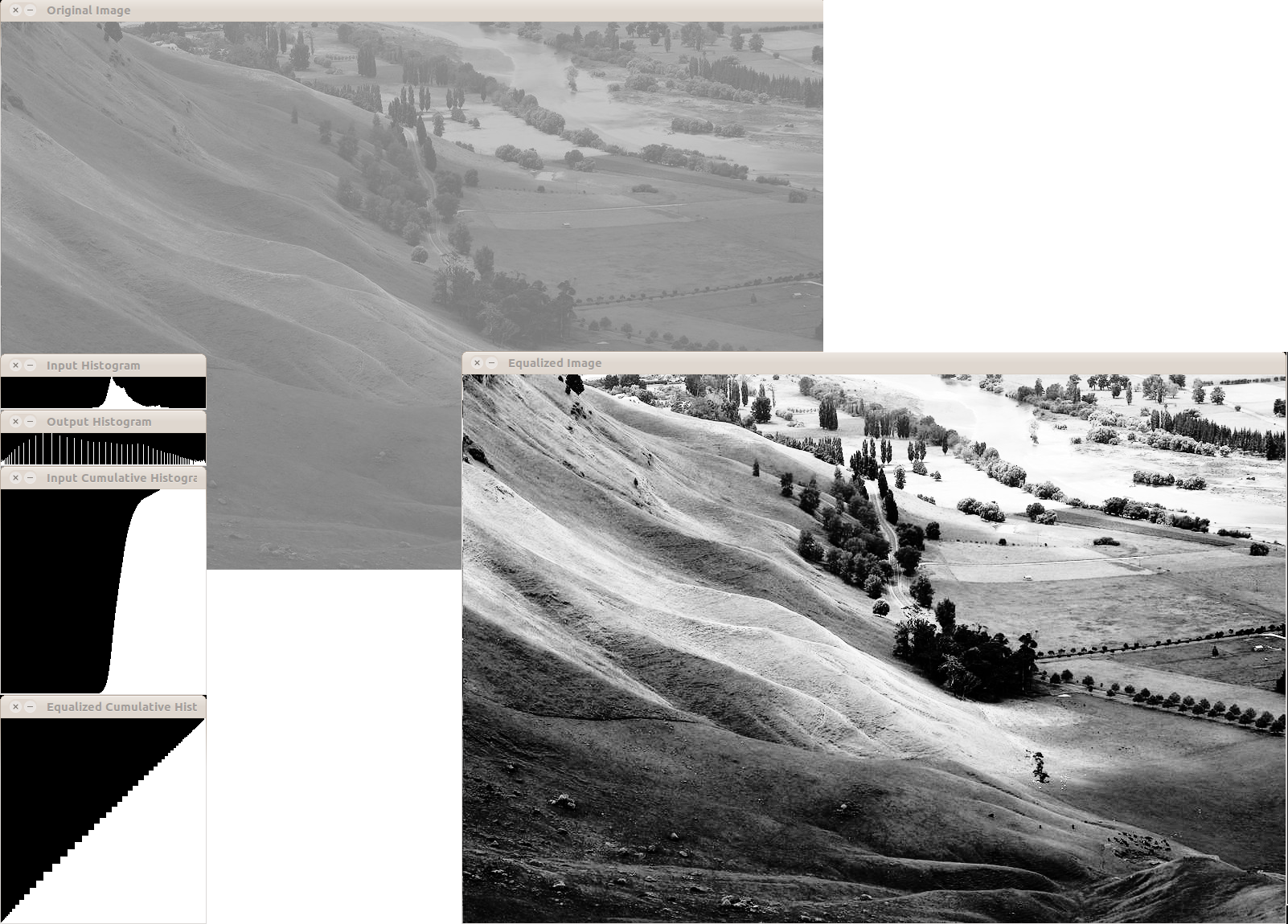
Fig. 1: An example of histogram equalization. Notice the input and output histograms and cumulative distribution functions.